R Bootcamp - Lecture 3 by Tengyu, Dash, Taylor, Milton and Bingjie

Data Wrangling

What is data wrangling? Data wrangling is the process of Data wrangling is the process of transforming and structuring data from one raw form into a desired format.

dplyr

dplyr is a package for data manipulation, written and maintained by Hadley Wickham. dplyr is a grammar of data manipulation, providing a consistent set of verbs that help you solve the most common data manipulation challenges.

To install dplyr package, run the following code in your R console:

install.packages("dplyr")

After installing the package, you can load it into your R session by using the following code:

library(dplyr)

Pipe Function

Pipe function is a very useful function in dplyr package. It looks like this: %>%. It is used to chain multiple functions together. Here is how your code looks like without pipe function:

filter(arrange(select(mtcars, cyl, mpg), cyl), mpg > 20)

Here is how your code looks like with pipe function:

mtcars %>% 
  select(cyl, mpg) %>% 
  arrange(cyl) %>% 
  filter(mpg > 20)

As you can see, the code with pipe function is much more readable. The pipe function takes the output of the function on the left side and feed it to the function on the right side.

Summarize

Summarize your data is an important step in data wrangling. It helps you to get a quick overview of your data. In dplyr package, you can use summarize function to summarize your data. Here is an example of calculating the mean calories using our cereal dataset(You can find it in the resources folder):

# Reading the cereal data:
df <- read.csv("cereal.csv")

df %>% summarise(avg = mean(calories))

Here's how the summarise function works:

First, you need to specify the dataset you want to summarize. In this case, it is df.
Then, you need to specify the variable you want to summarize. In this case, it is calories.
Finally, you need to specify the function you want to use to summarize the variable. In this case, it is mean.
We assign the result to a new variable called avg.

Summarize by group

Many times we want to compare the summary statistics of different groups. For example, we want to compare the average calories of cereals in different shelves. In this case, we can use group_by function to group the cereals by their shelves and then use summarise function to calculate the average calories of each group:

df %>% 
  group_by(shelf) %>% 
  summarise(avg = mean(calories))

We can also have multiple grouping variables. For example, we want to compare the average calories of cereals in different shelves and different manufacturers. In this case, we can use group_by function to group the cereals by their shelves and manufacturers and then use summarise function to calculate the average calories of each group:

df %>% 
  group_by(shelf, mfr) %>% 
  summarise(avg = mean(calories))

Summarize functions

There are many functions you can use to summarize your data. Here is a table of commonly used functions:

Function	Description
`mean()`	Mean
`median()`	Median
`sd()`	Standard deviation
`var()`	Variance
`min()`	Minimum
`max()`	Maximum
`sum()`	Sum
`count()`	Count
`n()`	Number of observations
`n_distinct()`	Number of unique values

Summarize multiple statistics

We can also summarize more than one statistics. For example, we want to calculate the mean and standard deviation of calories:

df %>% 
  summarise(mean = mean(calories), sd = sd(calories))

In the code, we use summarise function to calculate the mean and standard deviation of calories. We assign the result to two new variables called mean and sd.

Here's a snippet of code using group_by and summarise function. Try to figure out what it does:

df %>% 
  group_by(shelf, mfr) %>% 
  summarise(avg = mean(calories), cnt = n())

Manipulate columns

select

To select columns, we can use select function. Here is an example of selecting the first 5 columns of the cereal dataset:

df %>% 
  select(1:5)

We can also select columns by their names. Here is an example of selecting the mfr and calories columns:

df %>% 
  select(mfr, calories)

mutate

To create new columns, we can use mutate function. It's very important to note that mutate function will not change the original dataset. It will create a new dataset with the new columns. Here is an example of creating a new column called high_calories which is TRUE if the calories is greater than 100 and FALSE otherwise:

df %>% 
  mutate(high_calories = calories > 100)

In more complicated cases, we can define a vectorized function to calculate the new column. Here is an example of creating a new column called calories_3cat which is high if the calories is greater than 100, medium if the calories is between 50 and 100, and low otherwise:

calories_class <- function(calories){
    if(calories < 80){
      return('Low')
    } else if(calories < 120){
      return('Med')
    } else{
      return('High')
    }
  }
  calories_class_vec <- Vectorize(calories_class)
  df %>% mutate(c_class = calories_class_vec(calories))

rename

To rename columns, we can use rename function. It's very straightforward. Here is an example of renaming the mfr column to manufacturer:

df %>% 
  rename(manufacturer = mfr)

Note that on the left side of the = sign is the new name and on the right side is the old name.

Manipulate rows

filter

We use function filter to filter rows by certain conditions. Here is an example of filtering cereals with calories greater than 130:

df %>% 
  filter(calories > 130)

We can also have multiple conditions. For example, if you want to filter cereals with calories greater than 130 and sugars greater than 10, just add another condition and separate them with a comma:

df %>% 
  filter(calories > 130, sugars > 10)

arrange

Function arrange is used to sort rows. It can be used to sort rows by one or multiple columns, in ascending or descending order. By default, it sorts rows in ascending order. Here is an example of sorting cereals by calories

df %>% 
  arrange(calories)

To sort rows in descending order, we can use desc function.

df %>% 
  arrange(desc(calories))

To sort rows by multiple columns, we can just add more columns to the arrange function and separate them with a comma. Here is an example of sorting cereals by calories and sugars:

df %>% 
  arrange(calories, sugars)

distinct

Function distinct is used to remove duplicate rows or getting the unique values in columns. To remove duplicate rows in the whole dataframe, we can use distinct function without specifying any columns. Here is an example of removing duplicate rows in the whole dataframe:

# Data
df_dup <- data.frame(
Name = c("Alice", "Bob", "Charlie", "Alice", "David", "Bob", "Eve"),
Age = c(25, 30, 35, 25, 40, 30, 45),
Gender = c("F", "M", "M", "F", "M", "M", "F")
)

# Remove duplicate rows
df_dup %>% 
  distinct()

It can also be used to get the unique values in a column. For example:

df_dup %>% 
  distinct(Gender)

If we want to remove duplicate using a subset of columns, we can specify the columns in the distinct function and set .keep_all = TRUE. Here is an example of removing duplicate rows using a subset of columns:

df_dup %>% 
  distinct(Name, Age, .keep_all = TRUE)

Pivot table

For those who are familiar with Excel, you may know what a pivot table is. A pivot table is a table of statistics that summarizes the data of a more extensive table. In R, we can use tidyr package to create pivot tables. Here is an example of creating a pivot table using our cereal dataset:

library(tidyr)
df %>% 
  pivot_wider(names_from = mfr, values_from = calories)

Unpivot/melt table

Unpivot table is the opposite of pivot table. It is used to transform a pivot table back to the original form. In R, we can use the pivot_longer function in tidyr package to unpivot a table. Here is an example of unpivoting the pivot table we created in the previous section:

df %>% 
  pivot_wider(names_from = mfr, values_from = calories) %>% 
  pivot_longer(cols = c("A", "G", "K", "N", "P", "Q", "R"), names_to = "mfr", values_to = "calories")

Joining tables

Many times, the data we want to analyze is stored in multiple tables. In this case, we need to join the tables together. In this case the two or more tables share a common column. For example, we have a table containing student information and another table containing student grades. Joining the two tables together will give us a table containing both student information and student grades.

There are six types of joins in total: inner join, left join, right join, full join, semi join, and anti join. Here we will only talk about left join and inner join since they are the most commonly used ones.

Left join

A left join will keep all the rows in the left table and join the rows in the right table that match the key. As shown in the figure below.

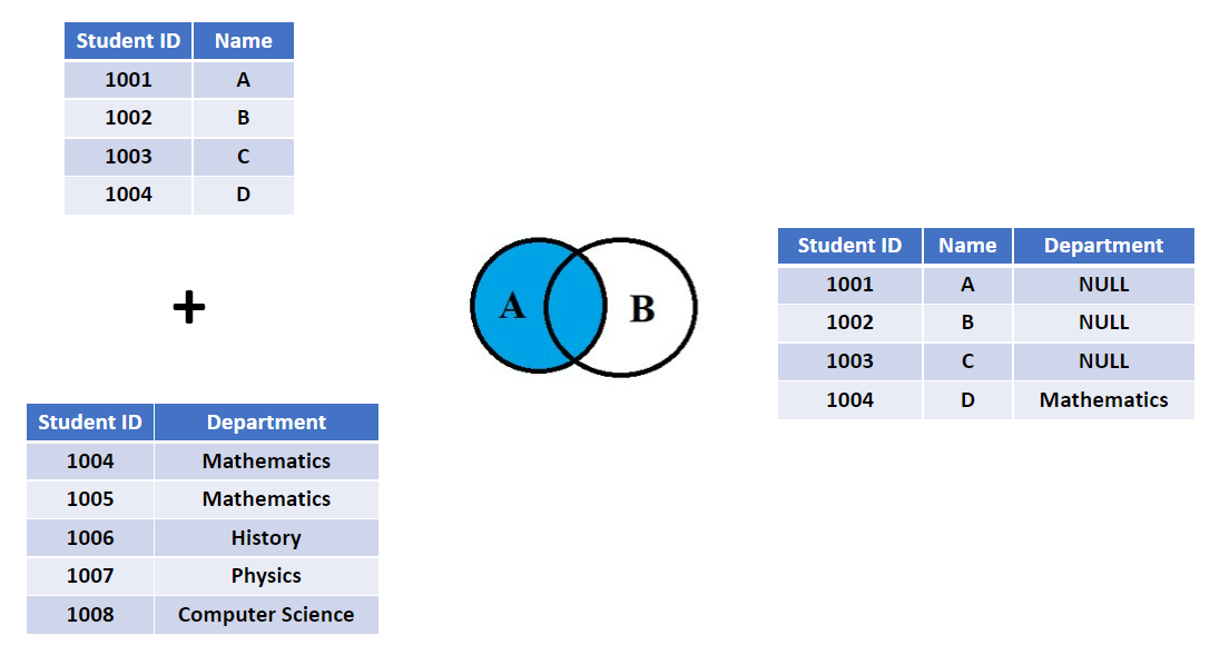
To show how to do a left join in R, let's first define the two table we are going to join:

# Data
df_stu <- data.frame(
  ID = c(1, 2, 3, 4),
  Name = c("Alice", "Bob", "Charlie", "David")
)

df_score <- data.frame(
  ID = c(3, 4, 5, 6),
  Score = c(85, 90, 80, 88)
)

Then we can use left_join function to join the two tables together:

df_stu %>% 
  left_join(df_score, by = "ID")

Inner join

Compared to left join, an inner join will only keep the rows that match the key in both tables. As shown in the figure below.

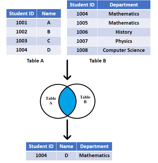
To do an inner join in R, we can use inner_join function:

df_stu %>% 
  inner_join(df_score, by = "ID")

As we can see, the result of inner join is different from the result of left join.

Handling missing value

Missing value is a common problem in data analysis. In R, missing value is represented by NA. In this section, we will talk about how to handle missing value in R.

Remove rows with NA

The first idea is to just remove the rows with missing value. In R, we can use drop_na function in tidyr package to remove rows with missing value.

We first define a dataframe with missing value:

# Data
df_missing <- data.frame(
  ID = 1:6,
  Value = c(10, NA, 15, NA, 20, 25)
)

Then we can use drop_na function to remove rows with missing value:

df_missing %>% 
  drop_na()

Filling with last value

Another way to deal with missing value is to fill it with the last value. For example in the table shown below.

Question	Category	Answer
Favorite movie	horror	Silent Hill
	comedy	American Pie
Favorite song	pop	Blank Space
	rock	Bohemian Rhapsody

In this example the first column has missing value. We can fill the missing value with the last value above it. The result will look like this:

Question	Category	Answer
Favorite movie	horror	Silent Hill
Favorite movie	comedy	American Pie
Favorite song	pop	Blank Space
Favorite song	rock	Bohemian Rhapsody

To perform it in R, we can use fill function in tidyr package. We continue to use the dataframe we defined in the previous section:

df_missing %>%
    fill(Value, .direction = "down")

Replace NA with arbitrary value

Another way to deal with missing value is to replace it with an arbitrary value. For example, we can replace the missing value with 0. The replace_na function in tidyr package can help us to do that.

df_missing %>% 
  replace_na(list(Value = 0))

Put it all together

Now let's put everything we learned together to build a data wrangling pipeline. Here is an example code. Can you tell what each line of coding is doing?

P.S. We are using the cereal dataset in this example.

df %>%
    filter(!mfr %in% c('N', 'Q')) %>%
    group_by(shelf) %>%
    summarise(Avg_carb = mean(carbo), Num = n()) %>%
    arrange(desc(Avg_carb)) %>%
    mutate(Total_carb = Avg_carb * Num) %>%
    rename(ShelfNo = shelf)

Cheat Sheet Resources

Tidyr cheatsheet: Link
Dplyr cheatsheet: Link

Some comments in the end

The syntax of tidyverse packages are verbose but intuitive. Sometimes when you are dealing with very large datasets and want faster speed, datatable will be a good choice.

In today's lecture: