R Bootcamp - Lecture 1   by Tengyu, Dash, Taylor, Milton and Bingjie

Installing R

Go to https://cran.r-project.org/.

Windows Users

For Windows users select the 'Download R for Windows' link and then click on the 'base' link and finally the download link 'Download R 4.3.1 for Windows'. This will begin the download of the '.exe' installation file. When the download has completed double click on the R executable file and follow the on-screen instructions. Full installation instructions can be found at the CRAN website.

Mac users

For Mac users select the 'Download R for (Mac) OS X' link. Choose your .pkg file based on whether your mac is on Apple silicon or Intel chips.

Installing RStudio

Go to https://posit.co/download/rstudio-desktop/.

On the right side, should be presented with the appropriate link for downloading Rstudio, no matter what system you use. Click on this link and once downloaded run the installer and follow the instructions.

IDE layout

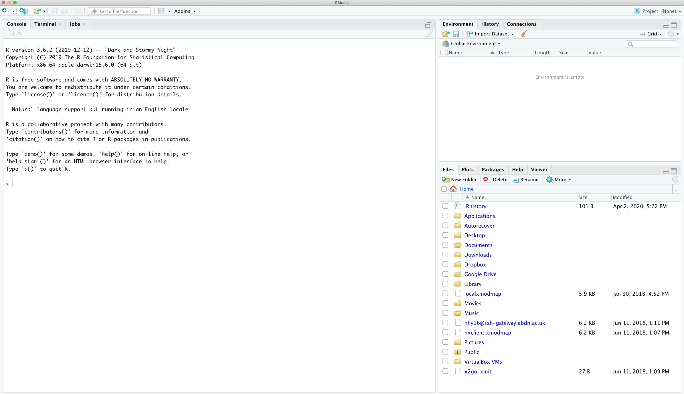
Console

Console is where R run all your codes and output the results. Let's try calculating 2+2 by typing it directly into console and hit enter.

Creating a R script

Instead of typing R code directly into the Console a better approach is to create an R script. R script is where you can write and store all your codes

Now your window should look like this.

Run lines in R script

To run lines from a R script, put your cursor on the line you want to run and click the run icon on top right.

There are other panels we haven't introduced yet. We will introduce when we need them.

R Markdown

R markdown is a great way to explore your data in an interactive way and output a well structured and replicable workflow. To start using Rmarkdown. Run the following commands in console.

install.packages("rmarkdown", dep = TRUE)

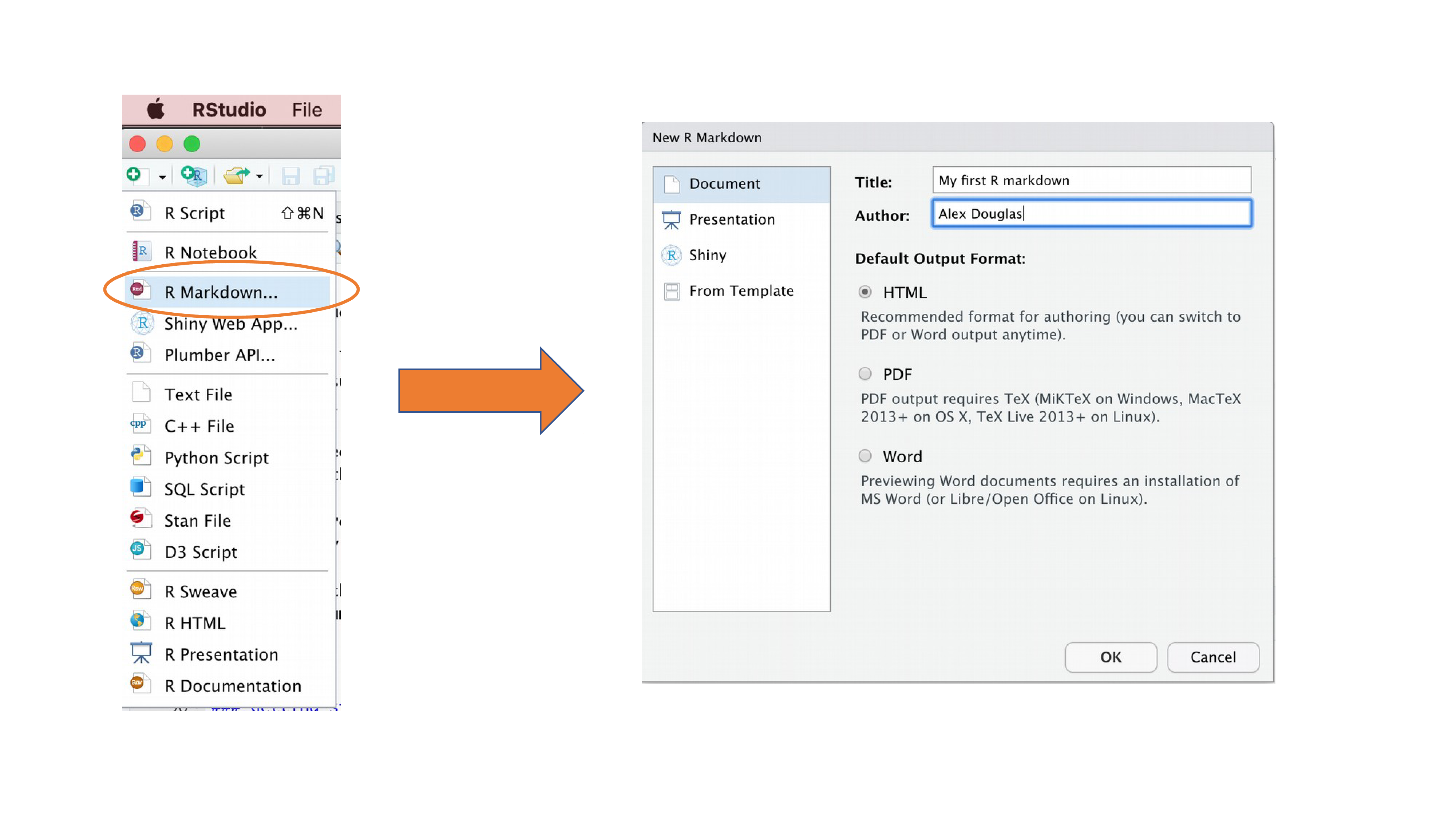
To create a markdown file, following the instruction from below

R markdown is basically markdown but with R code blocks in between. If you are unfamiliar with markdown. Here is some resources (https://www.markdownguide.org/basic-syntax/). To insert a code block. Put your cursor in the right place and click the insert icon on top right and choose R.

Basic syntax

Now let's try some basic syntax in R.

Assigning values to variables

Assigning values to variables is very easy. Just use the assignment operator <- or =. The variable name will be on the left side of the sign you choose and the value you want to assign to the variable should be on the right side of the sign.

variable1 <- 'Hello World!'
variable2 = 'HELLO WORLD!'
variable3 <- 12345

variable1
variable2
variable3

Printing

Use command print() or directly type out what you want to print. Use paste() or paste0() function to concatenate strings and variables.

print("Hello World!")
5 + 5

x <- 5
y = 6
x + y

text <- "Hello World!"

print(paste(text, x))
print(paste0(text, x))

Basic arithmetic operations & functions

• + (addition)
• - (subtraction)
• * (multiplication)
• / (division)
• ^ (exponentiation)
• == (equals to)
• %% (remainder)
• %/%(integer division)

x <- 2; y <- 3
x+y
x-y
x*y
x/y
x^y
x==2
2%%3
2%/%3

• abs(x) (absolute)
• sqrt(x) (square root)
• log(x) (ln(x))
• log10(x) (log of x based 10)
• exp(x) (e to the power of x)

x <- -25
y <- 25
abs(x)
sqrt(y)
log(y)
log10(y)
exp(2)

A little tip

If you are not sure what a function does, you can use ? or help() to get help.

?log
help(log)

Basic data types

• Character, such as 'hello world'
• Numeric, such as 10, 2.5, 3
• Logical, such as TRUE, FALSE

To check the data type of a variable, use class() function.

Use the is.num() / is.character() / is.logical() if you want a TRUE or FALSE value in return.

num <- 6
char <- 'abcdefg'
logi <- FALSE

is.numeric(num)
is.character(logi)
is.logical(logi)
class(num)
class(char)
class(logi)

Vectors

In R, we can assign vectors to variables using c():

• Numeric vectors: contains numeric values
• Character vectors: contains character values
• Logical vectors: contains logical values

x <- c(1, 2, 3, 4, 5)
y <- c(6, 7, 8, 9, 10)

x
y

# the operations are conducted element-wise
x + y

# It can also be a character vector
x <- c('1', '2', '3', '4', '5')
x

# or logical
x <- c(TRUE, FALSE, TRUE, FALSE, TRUE)
x

Note that when you try to have all three types of value in one vector, you will see that the values are all converted to character. Also, if only logical and numeric values are in a vector, the logical values will be converted into numeric values, with TRUE = 1 and FALSE = 0.

x <- c(1,'abc', FALSE)
x
y <- c(FALSE, 200)
y

Accessing Values in Vectors

Unlike other programming languages, indexing in R is very intuitive:

• The first element having the index '1'.
• The second element having the index '2'.
• The last element having the index which is the length of the vector length(name).

x <- c(100,200,300,400,500,600)
x[1]
x[length(x)]

Matrices

In R, we can create a simple matrix using the following: matrix(data, nrow = row_count, ncol = column_count)

x <- matrix(c(1, 2, 3, 4, 5, 6), nrow = 2, ncol = 3)
x

Note that the data will fill up the columns by default. If you want to fill up by row, modify the code as: matrix(data, nrow = row_count, ncol = column_count, byrow=TRUE)

x <- matrix(c(1, 2, 3, 4, 5, 6), nrow = 2, ncol = 3, byrow=TRUE)
x

Every element in a matrix must be of the same data type.

Also The dimension of the data must match the nrow and ncol you assign. You can just specify one of the nrow and ncol.

To perform matrix multiplication, use %*% sign.

To transpose the matrix, use t() (don't forget to assign the transposed matrix to a new variable!)

To access values in a matrix, use the same syntax as accessing such in vectors, except that you need to specify the row number and the column number.

y <- matrix(c(1, 2, 3, 4, 5, 6), nrow = 3, ncol = 2)
x%*%y
x[1,2]
t(x)

Dataframes

Dataframes are the most commonly used data type in R. They are similar to tables in Excel. They are two-dimensional arrays of data. The elements in a data frame can be of different data types.

df <- data.frame(name = c("John", "Mary", "Peter"), age = c(20, 21, 22), score = c(100, 90, 80))
df

There are many ways you can access values in a dataframe. Here are some examples.

• Accessing a column: Use the $ sign or the [,col_number], where [,col_number] is the column number you want to access.
• Accessing a row: Use the [row_number,], where [row_number,] is the row number you want to access.
• Accessing a value: Use the [row_number, col_number], where [row_number, col_number] is the row number and column number you want to access.
• Accessing a continous slice of values: Use the [row_number1:row_number2, col_number1:col_number2], where [row_number1:row_number2, col_number1:col_number2] is the row number and column number you want to access.
• Accesssing not continous values: Use the [c(row_number1, row_number2, ...), c(col_number1, col_number2, ...)], where [c(row_number1, row_number2, ...), c(col_number1, col_number2, ...)] is the row number and column number you want to access.

df$name
df[,1]
df[1,]
df[1,2]
df[1:2,1:2]
df[c(1,3),c(1,3)]

Factors

Factors are used to represent categorical variables with limited number of unique values. Like " Male" or "Female"

It is the default data type for categorical variables in dataframe.

x <- factor(c("alpha", "alpha", "beta", "gamma", "beta"))
x
levels(x)

Reading Data

There are many ways to read data in R. Here we show how to read data from a CSV file, an Excel file.

You will need to use the path to the file on your computer, or on the Internet.

If you don't know how to get the path to the file...

1. For windows users, just click the top bar of your file explorer and copy it.
2. For Mac users, right click on the file, hold Option and select "Copy ... as pathname". Or you can press Option+Command+P to show the path bar, then right click and select "Copy ... as pathname"

CSV files

URL = "https://gist.githubusercontent.com/netj/8836201/raw/6f9306ad21398ea43cba4f7d537619d0e07d5ae3/iris.csv"
x <- read.csv(URL)

# or

x <- read.table(URL, sep = ",", header = TRUE)
head(x)

Excel files

install.packages("readxl")
library(readxl)
xlsx_example <- readxl_example("datasets.xlsx")
x <- read_excel(xlsx_example)
head(x)

Inspect your data

There are many ways to take look at your data. The easiest way is to click on the dataframe in Environment. It will show a table in a new tab.

Another way is to use head() and tail() to show the first and last 6 rows of the data, as we did in the last two examples

# You can control how many rows you want to show by changing the n argument
head(df, n = 10)
tail(df, n = 10)

You can also use summary to get a summary of your data and dim to get the dimension of your data.

summary(df)
dim(df)

If you want...

You can use file.choose() instead of path to file to select your file with a GUI. But you have to do it everytime you run the code.

x <- read.csv(file.choose())

A little tip

You can set the work directory to a folder to avoid typing long pathnames

setwd("C:/Users/username/Documents/R_lab_material")

Basic Graphing

Here we show you how to make some basic plots

• Use hist() to graph a histogram of your data.
• Use boxplot() to graph a box plot of your data.
• Use plot(x,y) to plot a scatter plot between x and y.
• Use abline() to add a line in your plot.

par(mfrow=c(1,3))
hist(x$sepal.length)
boxplot(x$sepal.length)
plot(x$sepal.length,x$sepal.width)
abline(v=6,col='red')
abline(h=3.25,col='blue')